 Gowt.dev
Ferranti Effect
Table of Contents
Introduction
The Ferranti effect is a phenomenon in which the voltage at the receiving end (load side) is greater than the voltage at the sending end (source or generating side) of a long transmission line or cable during light load or no load conditions. The rise in voltage is due to more reactive power being generated by the line capacitance in the power lines than the power being consumed.
The conductors in the transmission line are placed in closed proximity, especially in underground cables that develop capacitance between them. In fact, the transmission cable constitutes many shunt capacitors and series inductors equally distributed along the length of the cable. The capacitance increases with an increase in the length of the transmission line. The capacitors draw a large amount of charging current that flows through the whole length of the line. The capacitor generates reactive power that flows in opposite direction toward the source. The inductors in the line consume the reactive power causing a voltage drop across them. The voltage drop is in-phase with the sending voltage. Therefore the voltages add up and the receiving voltage is increased.
An example with both theoretical calculation and its corresponding simulation in software is provided below.
System Parameters
- System Voltage: $V = 400\,\mathrm{kV}$
- Line Length: $l = 300\,\mathrm{km}$
- Series Resistance: $R = 0.1\,\Omega/\mathrm{km}$
- Series Reactance: $X = 0.4\,\Omega/\mathrm{km}$
- Shunt Susceptance: $B_c = 3.6 \times 10^{-6}\,\mathrm{S/km}$
- Frequency: $f = 50\,\mathrm{Hz}$
Manual Calculation
For a line length of 300km, the positive sequence parameters are calculated to be
$$R_{\text{total}} = R \cdot l = 0.1 \cdot 300 = 30\,\Omega$$ $$X_{\text{total}} = X \cdot l = 0.4 \cdot 300 = 120\,\Omega$$ $$B_{\text{total}} = B_c \cdot l = 3.6 \times 10^{-6} \cdot 300 = 0.00108\,\mathrm{S}$$
Calculation of zero sequence parameters
The zero sequence parameters are approximately three times the positive sequence parameters, which is typical for transmission lines.
$$R_0 = R \cdot 3 = 0.1 \cdot 3 = 0.3\,\Omega$$ $$X_0 = X \cdot 3 = 0.4 \cdot 3 = 1.2\,\Omega$$ $$B_0 = B_c \cdot 3 = 3.6 \times 10^{-6} \cdot 3 = 10.8 \times 10^{-6}\,\mathrm{S}$$
The impedance and admittance of the transmission line are defined as:
$$Z = R + jX = 30 + j\,120$$ $$Y = G + jB = 0 + j\,0.00108$$
The receiving-end voltage ($V_R$ ) and sending-end voltage ($V_S$) are related by:
$$V_R = \frac{V_S}{A}$$ $$ A = 1 + \frac{ZY}{2} $$ $$ZY = Z \cdot Y = (30 + j120)(j0.00108) = -0.1296 + 0.0324j$$ $$\frac{ZY}{2} = -0.0648 + 0.0162j$$ $$A = 1 + \frac{ZY}{2} = 1 - 0.0648 + 0.0162j = 0.9352 + 0.0162j$$ $${|A|} = \sqrt{0.9352^2 + 0.0162^2} \approx 0.93534$$
The receiving-end voltage due to the Ferranti effect is:
$$V_S = 400\,\mathrm{kV} \quad \Rightarrow \quad V_R = \frac{V_S}{|A|} = \frac{400}{0.93534} = 427.6518\,\mathrm{kV}$$
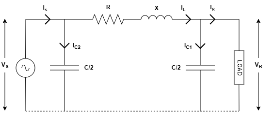
The transmission line is modelled as Nominal $\pi$. Here we are assuming, no load is connected to the line. The reactive power Q generated is directly proportional to the $V^2$ for a capacitive node.
$$\begin{align*} Q_R = \frac{V_R^2}{X_C} = V_R^2 \cdot B \end{align*}$$
Since the nominal $\pi$ method has half the capacitance in the end,
$$Q_R = \frac{V_R^2 \cdot B}{2} = \frac{427.6518^2 \cdot 0.00108}{2} = 98.7585\,\mathrm{Mvar}$$
To calculate the reactive power generated by the sending end capacitor,
$$\begin{align*} Q_S = \frac{V_S^2 \cdot B}{2} = \frac{400^2 \cdot 0.00108}{2} = 86.4\,\mathrm{Mvar} \end{align*}$$
$$\begin{align*} Q_{total} = Q_S + Q_R = 86.4 + 98.7585 = 185.1585\,\mathrm{Mvar} \end{align*}$$
To calculate the active and reactive power losses on the transmission line, we need to calculate the current. Since, no load is connected on the receiving end bus, we can take $I_R = 0$ and $I_L = I_{C1}$.
$$ I_{C1} = \frac{Q_R}{\sqrt{3} \cdot V_R} = \frac{98.7585}{\sqrt{3} \cdot 427.6518} = 0.133329\,\mathrm{kA} = 133.329\,\mathrm{A} $$
$$I_{C2} = \frac{Q_S}{\sqrt{3} \cdot V_S} = \frac{86.4}{\sqrt{3} \cdot 400} = 0.124708\,\mathrm{kA} = 124.708\,\mathrm{A}$$ $$I_S = I_{C1} + I_{C2} = 0.133329 + 0.124708 = 0.258036\,\mathrm{kA} = 258.036\,\mathrm{A}$$
Since $I_L=I_{C1}$ is the current flowing through $R$ and $X$, $P_{loss}$ and $Q_{loss}$ can be calculated by,
$$P_{\text{loss}} = 3 \cdot I_{C1}^2 \cdot R = 3 \cdot 133.329^{2} \cdot 30 = 1.599888 \times 10^{6}\,\mathrm{W} \approx 1.6\,\mathrm{MW} $$
$$Q_{\text{loss}} = 3 \cdot I_{C1}^2 \cdot X = 3 \cdot 133.329^{2} \cdot 120 = 6.39955 \times 10^{6}\,\mathrm{var} \approx 6.4\,\mathrm{Mvar}$$
The total reactive power injected into the grid can be found by,
$$ Q_{\text{grid}} = Q_{\text{total}} - Q_{\text{loss}} = 185.1585 - 6.4 = 178.7589\,\mathrm{Mvar} $$ Assuming the rated current of the transmission line is $1kA$,
$$Loading(\%)=\frac{I_{actual}}{I_{rated}} \cdot 100=\frac{0.258}{1} \cdot 100= 25.8\%$$
Simulation example
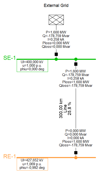
The same example with the given parameters is implemented in PowerFactory.
Conclusion
A comparison of the manual calculation and the simulated results is provided here.
| Parameter | Manual Calculation | Simulation Results |
|---|---|---|
| $V_S(kV)$ | 400 | 400 |
| $V_R(kV)$ | 427.6518 | 427.652 |
| $I_S(kA)$ | 0.258 | 0.258 |
| $P_{loss} (MW)$ | 1.6 | 1.6 |
| $Q_{grid} (Mvar)$ | 178.7589 | 178.759 |
| $Loading(\%)$ | 25.8 | 25.8 |